Documentation
The Electromagnetics (EM) solver is aimed at providing a powerful tool for simulating electromagnetic phenomena in the cloud. SimScale’s initial focus is centered around low-frequency domains, which include a major part of electromagnetic devices.
The current capabilities are matured around magnetostatic applications. This allows to investigate parameters such as magnetic flux density, magnetic field strength, current density, forces and torques, nonlinear materials, permanent magnets, inductances, and so on. Additionally, one can iterate on the design based on the simulation results and run as many simulations in parallel as needed.
In the near future, we plan to introduce additional modules that will enable simulations of AC magnetics, transient magnetics, electrostatics, AC electrics, and high-frequency applications at last.
The following information will explain the step-by-step procedure to set up an Electromagnetics simulation within the SimScale platform.
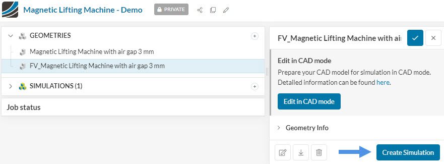
To create an electromagnetics analysis, first, select the desired geometry and click on ‘Create Simulation’:
Next, a window with a list of several analysis types supported in SimScale will be displayed:

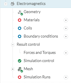
Choose ‘Electromagnetics‘ analysis type and click on ‘Create Simulation’. This will open the electromagnetics simulation tree which shows the steps needed to define the simulation.
To access the global settings, click on ‘Electromagnetics‘ in the simulation tree. In global settings, you can define the dominant field for your simulation.
We support magnetostatic, soon, more settings will be added to provide the user with options to run different types of electromagnetic problems.
The Geometry section allows you to view and select the CAD model required for the simulation. It is important that the CAD model is well-prepared to avoid any meshing or simulation-related errors. Find more details on CAD preparation and upload here.
In this step, users can define materials based on material properties associated with the analysis type chosen for the simulation. SimScale offers a default material library that enables a convenient and quick selection of materials. Additionally, users have the flexibility to create custom materials, which can then be saved in their personal material library for future use.
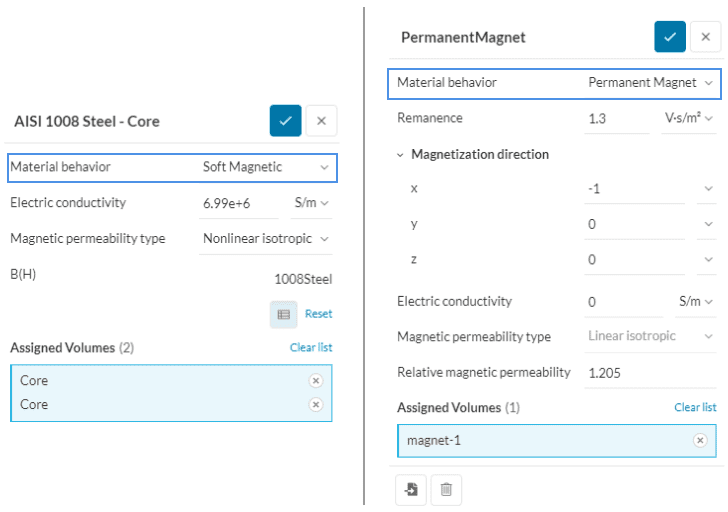
In a magnetostatic simulation, materials are differentiated based on their Material behavior, which can either be Soft Magnetic or Permanent Magnet. In both, the electrical conductivity and magnetic permeability of the material have to be defined. The Permanent Magnet definition also requires two additional inputs, which are the Remanence and the Magnetization direction of the permanent magnet.
In the following, a brief explanation of the terminology used for the material setup is provided.
Soft magnetic materials refer to substances that easily undergo magnetization and demagnetization processes, typically characterized by an intrinsic coercivity of less than 1000 \(\frac{A}{m}\). Intrinsic coercivity refers to the minimum magnetic field strength required to reduce the magnetization of a magnetic material to zero after it has been magnetized, indicating the material’s resistance to losing its magnetization.
These materials are primarily employed to enhance or direct the magnetic flux generated by an electric current. A key parameter for assessing soft magnetic materials is their relative permeability \(\mu_r\), which measures their responsiveness to an applied magnetic field.
Applications for soft magnetic materials can be categorized into two main types: Direct Current (DC) and Alternating Current (AC). In DC applications, the material is magnetized for a specific task and then demagnetized when the task is over. For example, an electromagnet of a lifting machine in a scrap yard is magnetized to attract scrap steel and demagnetized to drop the steel.
In AC applications, soft magnetic materials are repeatedly magnetized in different directions throughout their operational cycles, as seen in devices like power supply transformers. In both DC and AC applications, high permeability is desirable, but the significance of other material properties varies.
For DC applications, the primary consideration in material selection is often permeability, particularly in shielding applications where flux control is essential. Saturation magnetization may also play a role when the material is intended to generate magnetic fields or forces.
In AC applications, minimizing energy losses during the cyclic magnetization process is crucial. These losses can originate from three sources: hysteresis loss (related to the area within the hysteresis loop), eddy current loss (associated with electric currents induced in the material and resistive losses), and anomalous loss (linked to domain wall movement within the material).
Permanent magnets are fundamental components of modern technology, playing a pivotal role in various applications, from electric motors and generators to magnetic storage devices and medical imaging equipment. These materials exhibit a remarkable property: they possess a persistent magnetic field without the need for an external power source. This enduring magnetic field is what sets permanent magnets apart from temporary magnets, which only exhibit magnetic properties when exposed to an external magnetic field.
This property arises from the alignment of magnetic domains within the material, which remains fixed unless subjected to external factors such as high temperatures or strong opposing magnetic fields. Common materials used for permanent magnets include neodymium-iron-boron (NdFeB), samarium-cobalt (SmCo), and ferrite magnets.
Orientation and topology of permanent magnets
Currently, the magnetization direction can only be specified in cartesian coordinates with the ability to input custom vectors in case the magnet is not directly aligned. This implies that the magnetic field emitting from the surface of the permanent magnet is bound to be constant. Simulating permanent magnets with a curved topology (magnetic field tend to concentrate near curved region) will be possible in the near future.
Magnetic permeability, denoted by the symbol \(\mu\), is a measure of how easily a material can be magnetized in the presence of a magnetic field. It quantifies the material’s ability to support the formation of magnetic flux within itself when subjected to an applied magnetic field. Materials with high permeabilities allow magnetic flux through more easily than others.
Magnetic permeability is scalar if the medium is isotropic or a 3×3 matrix otherwise. Unlike electrical permittivity, permeability is often a highly nonlinear quantity, especially for steel and iron (ferromagnetic materials).
Mathematically, magnetic permeability is defined as the ratio of the magnetic flux density \(\textbf{B}\) to the magnetic field strength \(\textbf{H}\) within a material:
$$ \mu = \frac{\textbf{B}}{\textbf{H}} $$
Units of Measurement: The SI unit of magnetic permeability is Henry per meter \([\frac{H}{m}]\) or equivalently, Tesla meter per ampere \([\frac{T.m}{A}]\)
Types of Magnetic Permeability:
Since the permeability is a very small number, the relative permeability is the most commonly used parameter for material definitions.
In the setup, the user can choose the ‘Magnetic permeability type’ which can be either Linear Isotropic or Nonlinear Isotropic. In the prior, a constant value of the Relative magnetic permeability is defined, while for the latter a B-H curve can be uploaded.
Figure 6 illustrates a comparison between linear and nonlinear magnetic permeability material definitions.
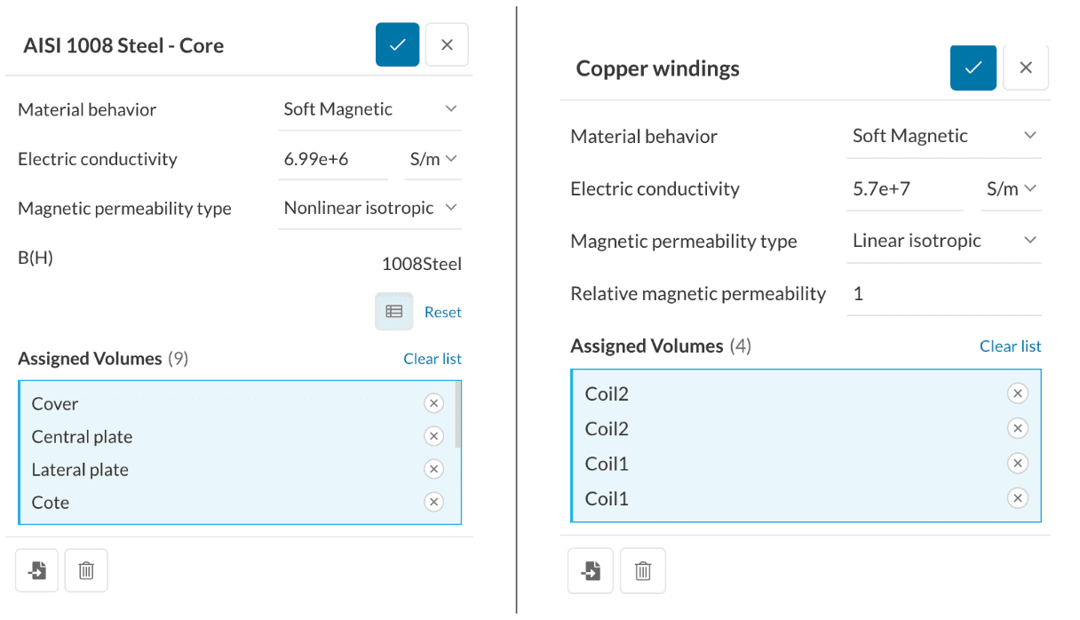
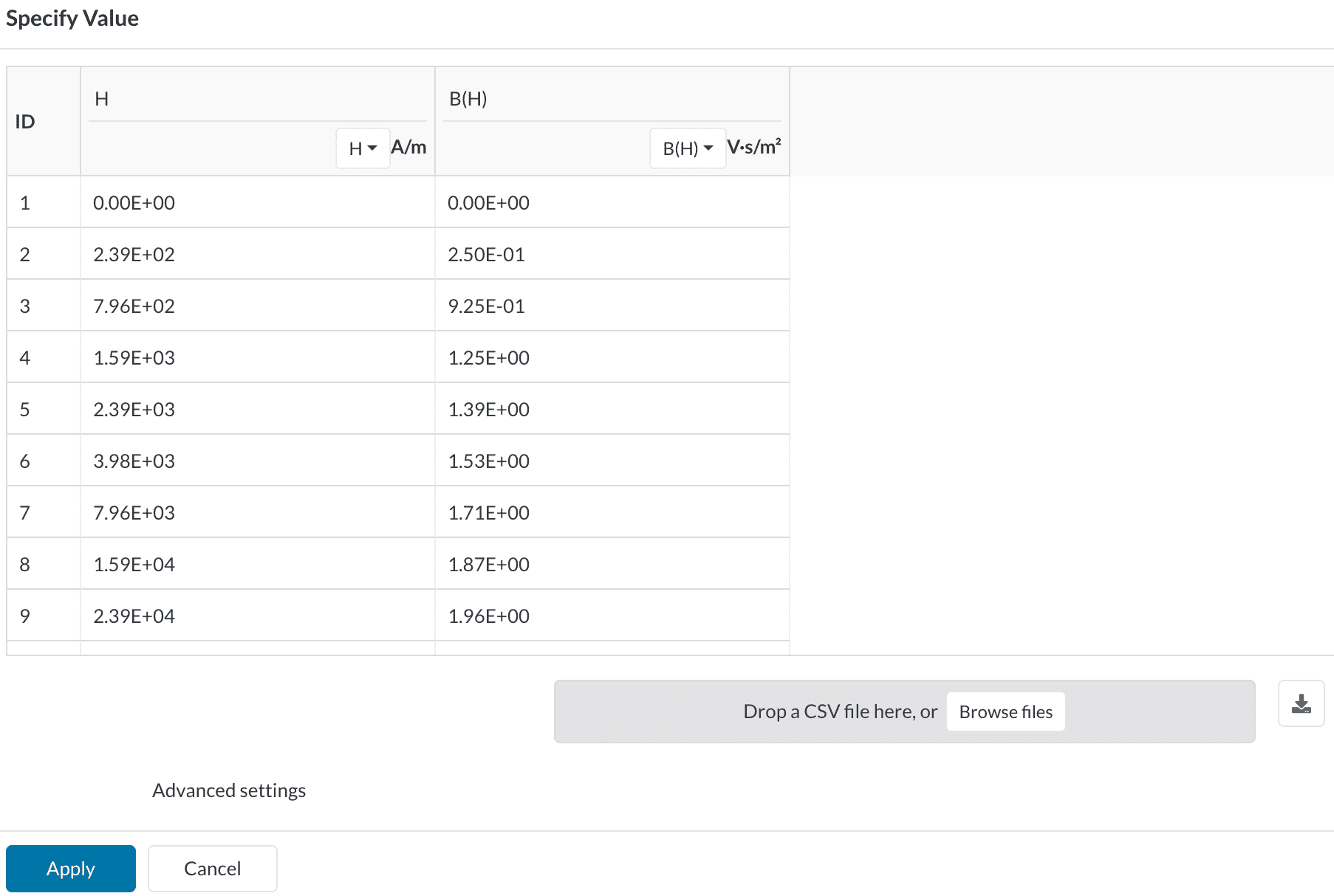
Figure 7 shows the table input for a nonlinear magnetic permeability. The units of \(\textbf{H}\) and \(\textbf{B}\) should be provided in SI units as \(\frac{A}{m}\) and \(T\) or \(\frac{V.s}{m^2}\), respectively.
Uploading \(\textbf{B}\)\(\textbf{H}\)-curve data
There are two main rules that need to be satisfied when importing \(\textbf{B}\)\(\textbf{H}\)-curve data:
Remanence (\(B_r\)) also known as retentivity or residual magnetism is a fundamental concept in the field of magnetism and materials science that describes the phenomenon whereby certain materials retain a permanent magnetization even after an external magnetic field is removed. This enduring magnetization arises from the alignment of magnetic moments within the material’s atomic or molecular structure. In simple terms, the higher the value of Remanence the stronger the magnet is.
For example, the magnetic memory in magnetic storage devices, as well as in everyday magnets or materials that can be easily magnetized, is a result of remanence. When there is a need to eliminate this remanence, it can be accomplished by subjecting the material to a negative inducing field, a procedure commonly referred to as degaussing.
The concept of remanence can be easier to understand through the magnetic hysteresis curve shown in Figure 8 below. The hysteresis curve illustrates the relationship between the magnetic field strength \(\textbf{H}\) and the resulting magnetic induction \(\textbf{B}\) in a material, showing how a material responds as it is magnetized and demagnetized.

In the case of a ferromagnetic material that has never been magnetized before or has been completely demagnetized, it will follow the dashed line when \(\textbf{H}\) is increased. This line shows that the higher the applied magnetizing force or current (\(\textbf{H}\)+), the stronger the magnetic field within the component (\(\textbf{B}\)+).
At point “a” almost all of the magnetic domains are aligned, and further increase in the magnetizing force will result in minimal additional magnetic flux. This marks the material’s state of magnetic saturation.
When \(\textbf{H}\) is reduced to zero, the curve shifts from “a” to “b.” At the intersection of the curve with point “b”, it’s evident that some residual magnetic flux \(\textbf{B}\) remains within the material despite a zero magnetizing force. This point is known as remanence or retentivity on the graph and signifies the material’s remanence or the degree of remaining magnetism (where some domains maintain alignment while others lose it).
As the magnetizing force is reversed, the curve progresses to point “c,” where the flux is reduced to zero. This is termed coercivity on the curve, indicating that the reversed magnetizing force has flipped enough domains to nullify the net flux within the material. The energy required to eliminate the remaining magnetism from the material is referred to as the coercive force or coercivity of the material.
Hard and soft magnetic materials on a hystersis curve
Typically, hard magnetic materials are commonly referred to as permanent magnets, and these materials exhibit a B-H Curve that commences in the second quadrant when displaying nonlinear behavior. On the other hand, there are magnets, distinct from permanent magnets, known as soft magnetic materials, whose B-H Curve is confined to the first quadrant.
Electrical conductivity, also known as specific conductance or simply conductivity, refers to the ability of a material to conduct an electric current. It is a fundamental property of materials that determines how easily electric charges can flow through them. Conductivity is typically measured in units of Siemens per meter \([\frac{S}{m}]\)
In a solid material, electrical conductivity is influenced by the movement of charged particles, such as electrons or ions. Metals are excellent conductors of electricity due to the presence of free electrons that are loosely bound to the atomic structure. When a potential difference (voltage) is applied across a metal, these free electrons can move freely and carry the electric charge, resulting in high conductivity.
In contrast, insulators have very low electrical conductivity because their electrons are tightly bound to the atomic structure, making it difficult for them to move. Examples of insulators include plastics, rubber, glass, and ceramics. These materials impede the flow of electric current, and their conductivity is typically negligible for practical purposes.
Semiconductors, however, have an intermediate level of conductivity that can significantly vary depending on factors such as exposure to electric fields or specific frequencies of light
Electrical conductivity finds application in analyses such as Electric Conduction, AC Magnetic, and Transient Magnetic studies.
A coil is a configuration where the length of the conductor, often copper wire, is wound multiple times around a central core. When an electric current flows through these windings, they collectively generate a magnetic field. This phenomenon forms the basis for various applications in electromagnetics.
In the context of coils, a notable distinction is drawn between two main categories: Solid coils and Stranded (wound) coils.
A Solid coil is crafted from a single continuous piece of conductor material, providing an unbroken path for electric current. As the current flows through this uninterrupted path, the current density—defined as the amount of current per unit cross-sectional area—can vary based on the conductor’s geometry. In Solid coils, irregularities in the conductor’s material or variations in its cross-sectional dimensions can lead to uneven current distribution and subsequently non-uniform current density.
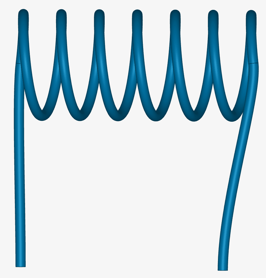
Conversely, a stranded coil refers to a volume modeling of a coil that is formed by wrapping multiple turns of a conductor, typically made of materials like copper wire, around a cylindrical core or bobbin. A Stranded coil definition allows the user to simplify the modeling approach of the actual stranded coil, by simply replacing the stranded coil wires with an equivalent size cross-section.
For example, Figure 10 below highlights the difference in modeling approaches between a complex and a simple stranded coil approach. In this example, two different electric motor geometries are shown. Where one is modeled with actual strands of wire, and in the other approach these strands are lumped together into an equivalent volume, in which later in the simulation setup the number of turns of the wire inside that volume would be specified.

Utilizing the Stranded coil type definition not only simplifies the geometry creation process but also leads to a reduction in both mesh element count and simulation computation time. This approach allows for the creation of a single or multiple-volume coil that mimics the behavior of being stranded, hence eliminating the need for manual strand-by-strand construction.
Moreover, if one was to go ahead with the complex stranded coil approach, then each strand of wire would need to be defined as a coil. In that case, the coil could be either defined as a solid coil, or a stranded coil with 1 turn. However, since there is a large number of coils that need to be defined, the complex approach would be significantly more time-consuming to set up than the simple stranded coil approach.
Moving on, the distinct current distribution in these coil types influences the resulting magnetic field. In a solid coil, the uneven current density can lead to non-uniform magnetic field generation, with stronger magnetic effects where the current density is higher and weaker effects where it’s lower. In contrast, the uniform current density in a Stranded coil produces a magnetic field that is generally more evenly distributed and consistent.
The total current flowing in a Stranded coil is simply the current per turn multiplied by the total number of turns: \(I = \frac{current}{turn} * N\)
In the case of a Solid coil, the total current is simply the net current \(I\) flowing through it. This means that in both stranded and solid coils, the net current would be the same in the end. If that is the case, one may wonder what is really the difference between solid and stranded coils when it comes to their applications in simulations.
The disparities between these coil types emerge based on the chosen type of analysis. Whether it involves Magnetostatic, AC magnetic, or Transient magnetic simulations, the distinctions become apparent.
In the study of Magnetostatics, there are no induced currents, and hence the total current in the coil is simply the applied current. As previously mentioned, the current density distribution in a stranded coil is uniform, however, it varies in a solid coil. Consequently, there can be a small difference in the magnetic field between the two. Inductances, on the other hand, would be completely different between solid and stranded coils since it depends on the number of turns.
The differences in the context of AC magnetic and Transient magnetic would be explained, once those solvers are released.
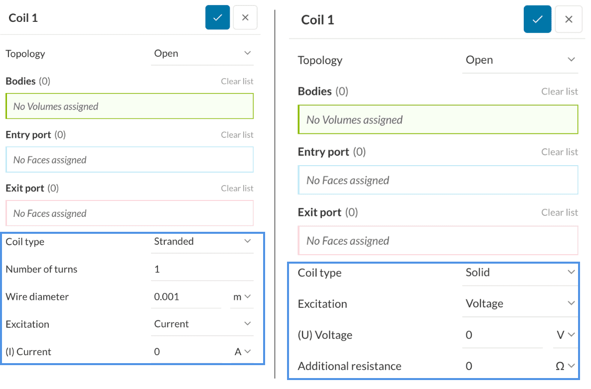
The setup of coils in SimScale revolves around two fundamental parameters: Coil type and Topology. These parameters determine how your coil will behave in the simulation.
Coil type
The Coil type parameter classifies coils into two categories: Solid and Stranded. This classification defines the coil’s structural composition and its subsequent behavior within the electromagnetic field.
In a Solid coil only the Excitation needs to be defined which can either be via a net (I) Current or a (U) Voltage, while for a Stranded coil, two additional parameters to the Excitation are required which are the Number of turns and Wire diameter.
Specifying current for multiple coil bodies in one coil setup
The current value specified for in a coil setup is averaged over the number of coil bodies inside that setup. For example, if you have a coil setup which has 4 coils defined inside it, meaning 4 entry and 4 exit ports or 4 internal ports. Then if the input current is 100 Amperes, this would result in each coil receiving a current value of 25 Amperes. If the intended current in each of the 4 coils was 100 Amperes, then the value given inside the coil setup should be 400 Amperes.
Parametric simulations
In the simulation, the current input is parameterizable. With parametric studies, the user can quickly set up, run, and compare results for several configurations in parallel saving heavily on computational time. Currently, SimScale supports only one parametric definition in the simulation seutp. Meaning, you would not be able to parametrize the current inputs for multiple coils.
Topology
The Topology parameter dictates whether your coil is characterized as Open or Closed. This defines whether the coil is modeled as a closed loop or has open boundaries.
In general, The net current does not give information about the direction of current flow in the coil. It is the current density that gives such information. Therefore, it is necessary to specify a port or a pair of ports that dictates the direction in which the current flows.
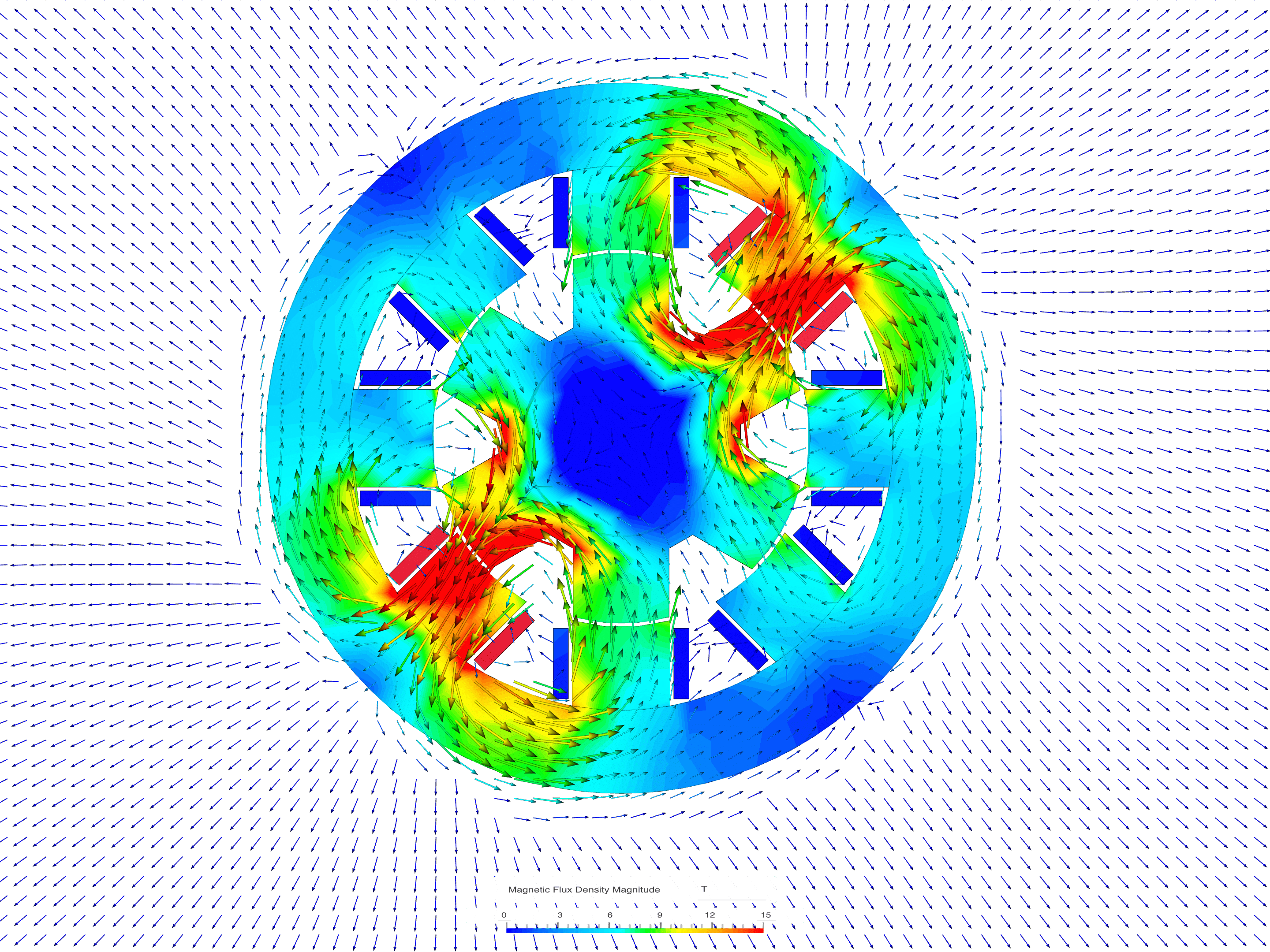
Figure 12 below compares the setup of an open coil (left) to the setup of a closed coil (right). Notice, in the open coil scenario, the coil has an open topology with clear entry and exit ports on the front and back sides of the motor. On the other hand, an internal port is chosen for the closed coil.

Boundary conditions help to add closure to the problem at hand by defining how a system interacts with the environment. There are currently two types of boundary conditions that are supported in the context of electromagnetics:

This boundary condition enforces the presence of a normal magnetic field \(\textbf{H}\), effectively nullifying any tangential magnetic field \(\textbf{H}\), across a given surface. The normal field must be applied on all faces belonging to a plane of symmetry where the magnetic field \(\textbf{H}\) is purely normal.
This boundary condition enforces the presence of tangential flux, effectively nullifying any normal flux \(\textbf{B}\), across a given surface. The Tangential flux must be applied on all faces belonging to a plane of symmetry where the magnetic flux density is purely tangential.
If a coil is in contact with the bounding box (e.g. air volume) boundary and if the current is flowing normal to that boundary, then a tangential flux boundary condition must be applied. In other words, if you have an entry or an exit port that is aligned with the outer boundary of the bounding box then assign a tangential flux boundary condition on all the faces on that boundary.
Note that when applying those boundary conditions they should be assigned on all faces of the external boundaries.
Why are the boundary conditions called Magnetic flux tangential and Magnetic field normal?
Simply because that is exactly what is prescribed in the equations. In the magnetic flux tangential BC the normal component of the magnetic flux density is zero, and in the normal field BC the tangential component of the magnetic field is zero. Useful to know is that, for an isotropic material the flux tangential BC also means that the field is tangential, and the field normal BC also means that the flux is normal. However, in general (for anisotropic materials) this is not true. Hence, the naming is as such in order to maintain an accurate representation of the names.
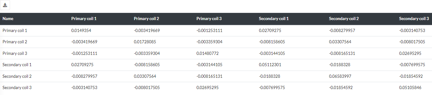
The Result Control section allows users to define additional simulation result outputs that aid in the analysis of the design. In the Electromagnetics simulation type, the additional outputs supported are the inductances, forces, and torques. The results of those parameters are provided in table format along with the coil resistance values and can all be accessed under the Tables item after the simulation is completed.
The phenomenon of creating an electric current within a conductor through exposure to a changing magnetic field is referred to as electromagnetic induction, or simply, induction.
The term “induction” is used because the magnetic field is responsible for inducing the current within the conductor. The Simwiki article here provides a detailed description of the concept of electromagnetic induction.
Inductance signifies an inductor’s capacity to store energy within the magnetic field which results from the movement of electric current. The establishment of this magnetic field demands energy input, which is subsequently discharged upon the field’s loss of strength.
Understanding the impact of inductance becomes clearer with a simple loop of wire as an example. Imagine applying a sudden voltage across the wire loop’s ends. In response, the current needs to shift from zero to a nonzero value. However, a nonzero current generates a magnetic field following Maxwell-Ampere’s law.
As the current rises to its stable value as determined by Ohm’s law \(I = \frac{V}{R}\) the magnetic field it generates gradually takes on its steady form. Since the magnetic field is changing in the process, it induces a voltage in the coil itself—a phenomenon consistent with Lenz’s Law. This induced voltage is also termed back electromotive force (back EMF). The strength of this emf depends on the rate of change in current and the inductance.
When electromagnetic induction takes place within an electrical circuit and influences the flow of electricity, it is termed inductance, denoted as \(L\). The unit of inductance is Henry \(H\).
There are two types of inductances:
In a system comprising N coils, the inductance is represented as an NxN matrix. Here, Lii signifies self-inductance, while Lij denotes mutual inductance. To facilitate this matrix representation, it’s essential to sequentially number the coils.
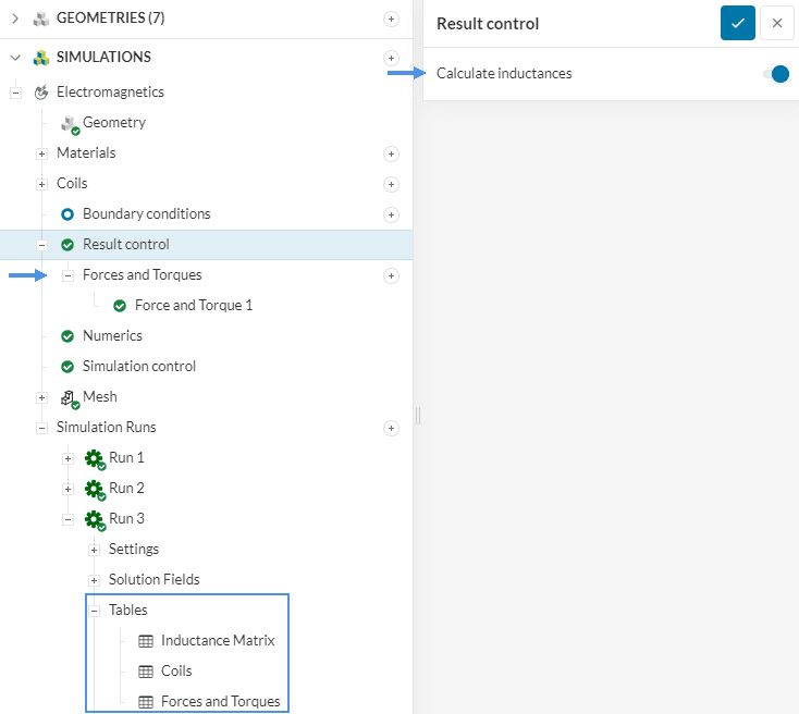
To enable inductance calculation in the simulation, click on the ‘Result control‘ item, and then a pop-up window will appear on the top right of the simulation tree as shown in Figure 14. Simply, activate the radio button to enable inductance calculation.
This Result control item calculates the Forces and Torques due to the electromagnetic field on a specified volume (part).
The forces and moments calculation is based on the virtual work method. This approach involves determining the change in the overall magnetic energy as the object is moved a distance \(\Delta s\) along the direction of the desired force component.
This yields that the force along the displacement direction \(s\) is:
$$ F_s = \frac{W_2 – W_1}{\delta s} $$
Where \(W\) is the virtual work and can be computed as:
$$ W = \frac{1}{2} \int{B \cdot H \, dv} $$
The torque can be obtained by rotating the component by a differential degree \(\Delta \phi\) around any of the Cartesian axes:
$$ \tau = \frac{W_2 – W_1}{\Delta \phi} $$
To define a Forces and Torques output, you can simply access it under the Result control item as shown in Figure 14. Then the user is prompted to choose a volume on which the Forces and torques would be calculated. For the Torque calculation, a Torque Reference Point needs to be defined.

Useful to know about the virtual work method
In order to obtain accurate results when using the virtual work method, it is important that the body on which the forces and torques are calculated on, is surrounded by force-free materials (e.g. air). Force-free materials are substances that neither exert forces on electric charges nor interact with magnetic fields. They are typically insulators, no current flows through them, and have a magnetic permeability equal to that of free space.
Numerical settings play an important role in the simulation configuration. They define how to solve the equations by applying proper discretization schemes and solvers to the equations. They help enhance the stability and robustness of the simulation.
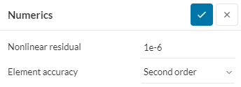
The Element accuracy setting allows the user to choose the order of the finite element, a selection between first-order (linear shape functions) and second-order (parabolic shape functions) is available.
The default Element accuracy is second order. It is recommended to leave it as such when higher accuracy is desired, especially when calculating forces and torques. The second-order element, while more accurate, does come with higher computational demands compared to the first-order element due to the additional degrees of freedom in the elements.
This represents the maximum permissible error in the iterative solver. When dealing with a well-defined model, the iterative solver will continue its iterations until it achieves an error lower than this specified value. Should it be unable to attain an error smaller than this threshold, it will terminate and report a failure. The smaller the nonlinear residual value the tighter the convergence of the simulation will be, which can result in a more accurate solution at the expense of an additional solving time.
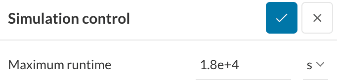
The Simulation control settings define the general controls over the simulation. Users can define the Maximum runtime of the simulation here which dictates the maximum runtime of your simulation in real-time. The simulation run stops when it goes beyond this value.
Meshing is the process of discretization of the simulation domain. That means we split up a large domain into multiple smaller domains and solve equations for them.
For an electromagnetic analysis, the standard algorithm is available. For more information about meshes, make sure to check the dedicated page.
References
Last updated: January 8th, 2024
We appreciate and value your feedback.
Sign up for SimScale
and start simulating now